Evaluating the Power of Predictive Analytics: Statistics Basics for Clinicians and Quality Professionals

Imagine your health care organization is challenged with excess readmissions to the hospital. Suddenly, you find yourself on a vendor selection team to evaluate predictive analytics that will help your care management team be more proactive in transition of care planning for your patients. 

Predictive analytics is the practice of extracting information from existing data sets in order to determine patterns and predict future outcomes and trends. Predictive analytics does not tell you what will happen in the future; rather, they forecast what might happen in the future with an acceptable level of certainty. Today, we’ll dive into four common statistics used to evaluate the strength of predictive analytics, which are increasingly being adopted by the health care industry.

Sensitivity and specificity are two statistical measures used to evaluate the performance of predictive analytics when the condition being predicted is either “true” or “false.” This is called a binary classification model, because there are only two possible outcomes. Sensitivity can be used to evaluate the ability of medical tests to correctly identify those with a disease (true positive rate). Specificity, on the other hand, is the ability to correctly identify those without the disease (true negative rate).

In a perfect world, both sensitivity (the accuracy of predicting yeses) and specificity (the accuracy of predicting nos) would both be 100% (expressed as 1.0). In the real world, however, there is no such thing as a perfect predictive model or medical test. Therefore, it is important to interpret both the sensitivity and specificity together when deciding on the power of a predictive analytic.

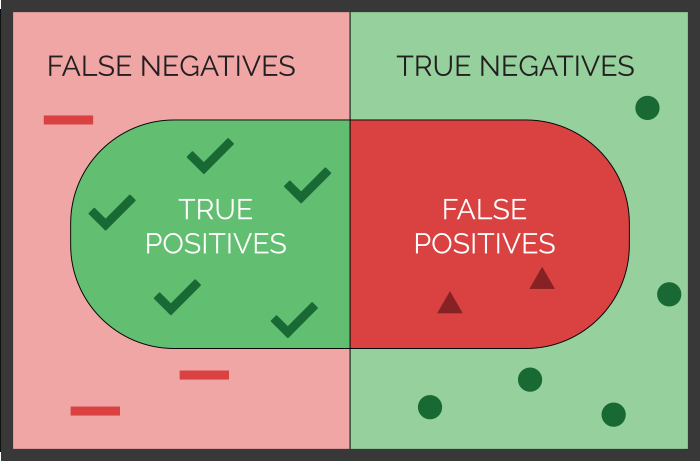
Figure 1 illustrates the concepts of sensitivity and specificity and their simple mathematical formulas. It’s almost like looking under a microscope, where you are examining the condition you are trying to predict. In this view you will see both true and false positives. The world around your microscope slide are the true and false negatives.
       

                                                                                                                               
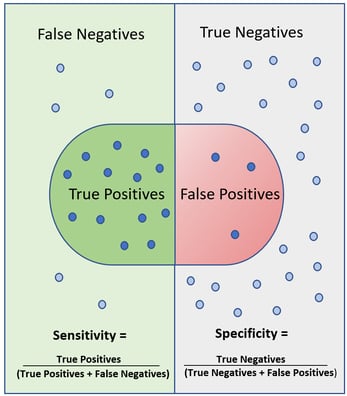
Figure 1. Sensitivity and Specificity 

Sensitivity is the true positive rate calculated as True Positives/ (True Positives + False Negatives). Sensitivity decreases when the number of false negatives increase. False negatives are known as Type II errors.

Specificity is the true negative rate calculated as True Negatives/ (True Negatives + False Positives). Specificity decreases when the number of false positives increases. False positives are known as Type I errors.

Precision, also known as the Positive Predictive Value (PPV) is a third statistic that typically accompanies sensitivity and specificity. Precision, or PPV, is calculated as True Positives/ (True Positives + False Positives). Precision decreases when there are more false positives predicted.

Precision is important to evaluate when the predictive analytic is deployed as an alert that requires attention or action by the receiver. Analytics with low precision can result in alarm fatigue and are typically less helpful over time. When evaluating precision, it is generally helpful to look at the ratio of the numbers in the numerator and denominator rather than the overall rate so that you can more easily understand the number of times you will receive a true alert out of all the alerts generated.

Prevalence is the fourth statistic that reflects performance of a predictive analytic. Prevalence is the number of times the phenomenon of interest occurs within the total population. Prevalence is calculated as True Positives + False Negatives/ Total population count. This statistic helps you prioritize the need for the predictive analytic in your organization.

The four statistics discussed above are often displayed in a table called a Confusion Matrix or a Contingency Table. Figure 2 illustrates a matrix for an analytic that is predicting which patients on a medical surgical unit are likely to “crash” and be transferred to a critical care environment or require emergency resuscitation. In this example, 1,000 patients on a medical surgical unit were evaluated. During this study period, there were 50 patients that required emergency intervention. Of these 50 patients, 31 patients were detected by the predictive analytic. However, the predictive alert failed to alarm on 19 patients that required emergency intervention. The sensitivity (ability to predict the patients that needed our help) was 31/ (31+19) = 62%. The specificity (ability to predict which patients would be ok and not need our help) was 700/ (700+250) = 74%. Finally, the precision was 31/ (31+250) = 11%, meaning that for every 281 alarms that went off, only 31 patients really needed our help! In this example, you can see how precision can determine if your staff will soon tire of responding to these alarms.

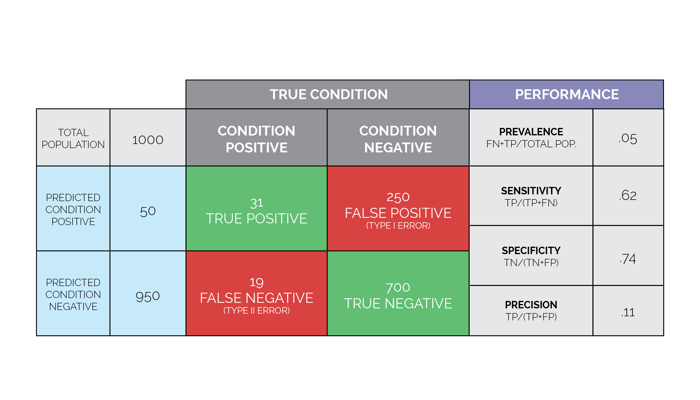Figure 2. Confusion Matrix (also known as Contingency Table)

Perhaps the most important formula to consider when deciding if predictive analytics are right for your organization is: IF you could know X, then you could DO Y. It isn’t enough to just implement predictive analytics. The stakeholders in your organization need to be clear and in agreement about the actions that will be taken when a predictive analytic is generated for a given patient or situation. Planning for the "Y" (expected actions) and evaluating the feasibility of potential interventions prior to deploying the "X" (predictive analytics) is an important step in the selection process and will add to the overall success of your investment. 

When working with vendors, it is often possible to “dial up” the sensitivity in order to capture fewer false negatives. Depending on what is at stake as a result of a false negative, you may wish to increase your sensitivity (ability to predict the yeses) at the cost of decreasing your specificity (ability to predict the nos).  Likewise, you may want to sacrifice sensitivity to increase specificity, resulting in fewer false positives. Finding the right balance between false negatives and false positives is key to successful adoption of predictive analytics in a clinical environment.

To find the optimal balance of sensitivity and specificity, ask the vendors you are evaluating whether they have two versions of the predictive analytics you are interested in. For example, a predictive model (also referred to as an algorithm) tuned for a very high sensitivity to identify patients at risk for new onset diabetes can be used for low-cost interventions, such as mailers or electronic surveys. The high sensitivity will ensure very few patients fall through the cracks. Then, use the algorithm tuned for high specificity for your higher cost interventions, such as biogenetic screening and intensive nutritional counselling and coaching for those patients who have the highest certainty of progressing to diabetes, while avoiding these costly services for those who are least likely to benefit. There will be relatively few false positives from this group of patients, so you can intervene with a high degree of confidence.

Finally, timing is everything when it comes to predictive analytics. An important question to ask your vendor is what the lead time is for the prediction being made and how often the prediction is updated or refreshed to detect changing conditions. This will largely depend on the source of data being used in the predictive models. It is possible to have predictive analytics that offer insight in a real or near real-time way as long as the algorithms use real or near real-time data from the EMR such as vital signs, laboratory results or medication orders. Retrospective data, such as ICD-10 diagnosis or CPT-4 procedure codes generated by the discharge abstract or billing system, are typically not available until two to five days after the patient is discharged unless you have real-time coding software. In the previous example for the detection of life-threatening conditions in medical surgical patients, a predictive analytic that generates an alert five minutes before a patient’s condition deteriorates will not provide enough time for an effective intervention to occur; whereas a lead time of 30 to 60 minutes would be more actionable. For predictive analytics to detect unplanned hospital readmissions, a lead time of one to two days prior to discharge would be optimally required.

Be sure to stay tuned for a future post where we'll uncover the mysteries of the C-statistic and other measures to evaluate correlations used in advanced analytics.